Synthetic Well Logging Platform · User Manual

Welcome to AILog

AILog lets you train neural networks on historical well log data (EDR, LWD, MWD) and produce synthetic logs, rock properties, and QC insights - all by dragging nodes onto a canvas and connecting them. No scripting required.

Tour the Interface

Build a Workflow

Browse Nodes

Try a Tutorial

What you can do

∑

Train Neural Networks

Use FFNN, LSTM, or TCN architectures to predict sonic, density, or any log curve from drilling and log inputs.

⟲

Generate Synthetic Logs

Apply trained models to blind wells to fill in missing log curves with uncertainty envelopes.

✓

Quality Control

Run QC passes on density, Vp/Vs, and mnemonics. Flag bad data before it enters your model.

⧉

Derive Rock Properties

Compute impedance, Vp/Vs ratios, UCS, and other elastic properties from your log suite.

The Interface

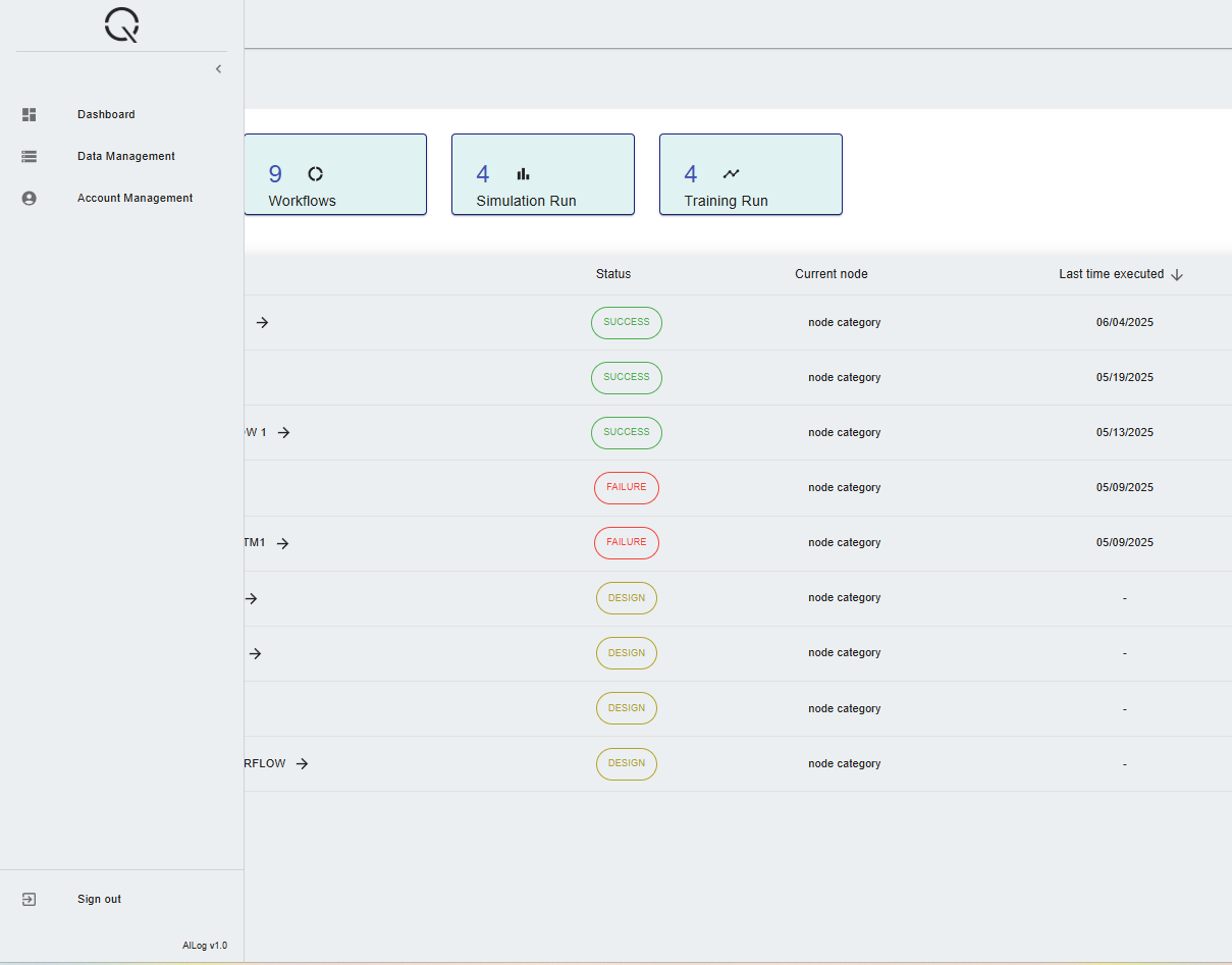
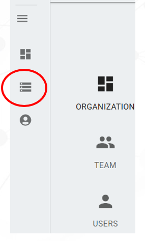
After you sign in, the left menu gives you three main destinations. You'll spend most of your time bouncing between Data Management and Workflow Dashboard.

MAIN TABS

DASHBOARD

DATA MANAGEMENT

ACCOUNTS

◎

Workflow Dashboard

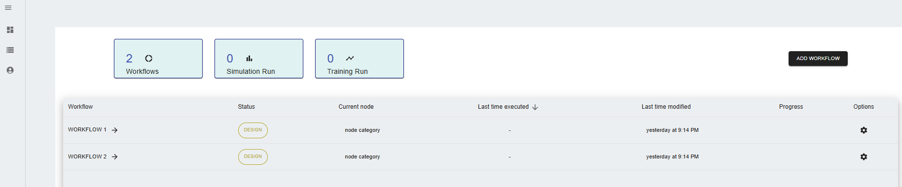
Lists every workflow you can see. Create new ones, open existing ones, or glance at completion counts and recent training runs.

▤

Data Management

A familiar file-tree for uploading, organizing, downloading, and deleting well data. Folders keep projects tidy.

⚿

Account Management

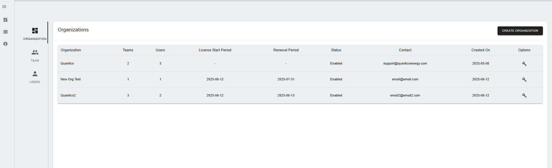
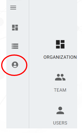
Manage organizations, teams, and users (admins only). Your personal profile and theme live in the top-right avatar menu.

Top bar & theme

User menu (top-right) - switch between dark and light theme, view profile, and log out.
Notifications - live toasts announce node completions, failures, and workflow events.
Breadcrumbs - inside a workflow, the top breadcrumb takes you back to the dashboard.

Account Management

Organizations hold Teams; Teams hold Users and own Workflows & Data. Who can see what depends on team membership.

The three roles

Role	Scope	Typical person
Super Admin	Every organization & team	Platform administrator
Admin	Multiple teams inside their organization	Team lead / project manager
Regular	One team	Petroleum engineer, data scientist

Creating an organization (Super Admin)

Open Account Management from the left menu.
Switch to the Organizations tab and click Add Organization.
Give the org a name and save. Each org is fully isolated - workflows, users, and data do not cross.

OVERVIEW

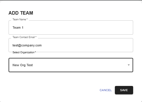
Adding a team

In Account Management, open the Teams tab.
Click Add Team, pick its parent organization, and give it a name.
Teams group both data and workflows. Users can belong to several teams.

TEAMS

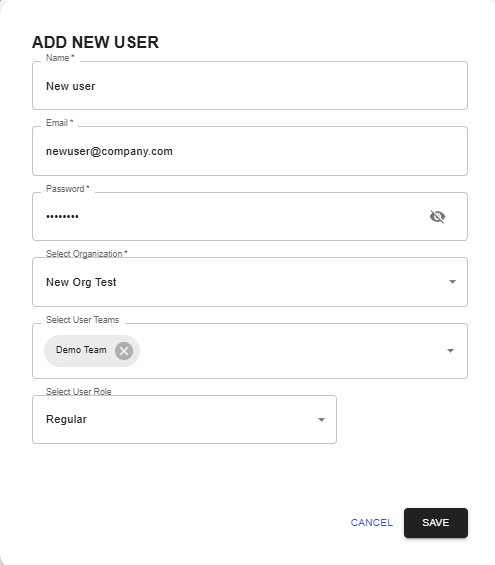
Adding a user

Open the Users tab and click Add User.
Fill in name, email, password, the team(s) they belong to, and role.
Regular users see only data and workflows in their team.

USERS

★

Plan your team layout before uploading data. Moving a dataset between teams later means re-uploading it.

Data Management

A familiar folders-and-files view. Everything that flows into a workflow starts here.

Supported formats

CSV - the most common input. Make sure the first row is headers (depth + mnemonics).
LAS - industry-standard log files. Units and mnemonics are parsed automatically.
XLS / XLSX - Excel spreadsheets. Headers in row 1.

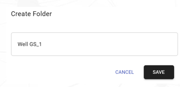
Creating folders

Open Data Management. If this is your first time, the view is empty.
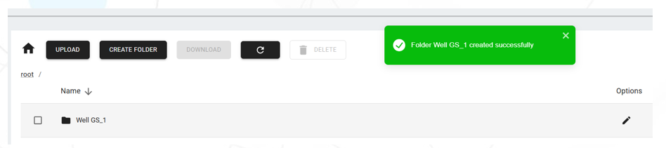
Click Create Folder. Enter a name (e.g. the well name or project name) and save.
A green toast confirms success. Click the folder to step into it.

CREATE FOLDER

STEP 1

STEP 2

Uploading files

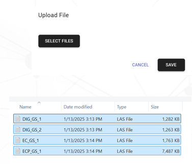
Inside the target folder, click Upload.
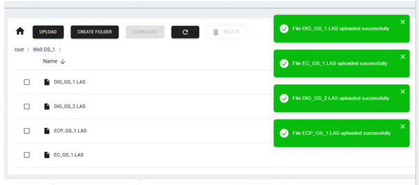
Click Select Files, choose one or many files, click Save.
Large files upload in multipart chunks; you'll see a progress bar. Don't close the tab until it finishes.

UPLOAD

FILES LOADED

Downloading & deleting

Download - works on single files or whole folders (zipped).
Delete - permanent. Removes the file from storage. Any workflow that referenced it will fail on re-run.
Rename - in-place, safe. Existing references update automatically.

Deleting a file in use breaks any workflow node currently pointing at it. Check dependencies before you delete.

Workflow Basics

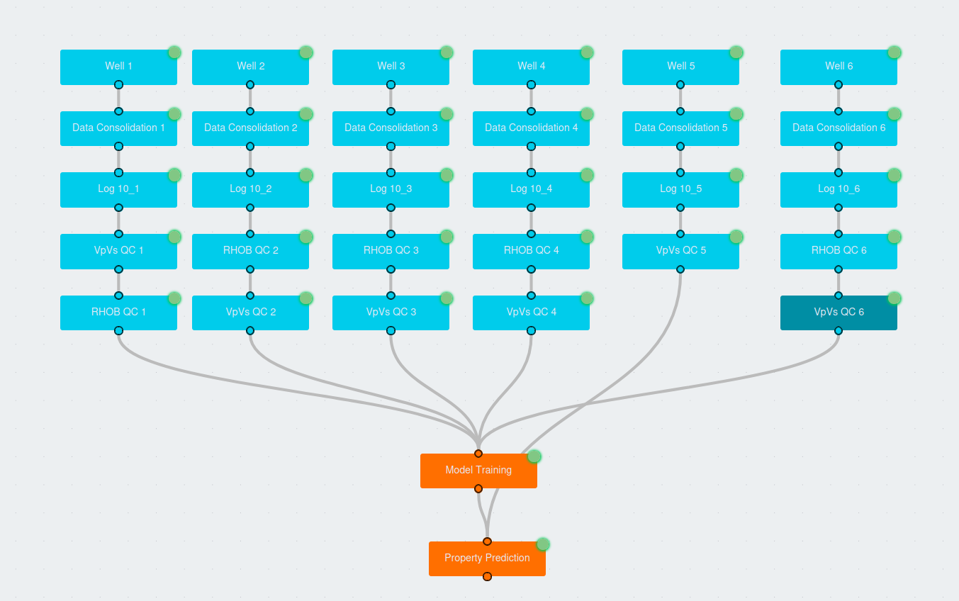
A workflow is a chain of processing nodes you build on the canvas. You drag, connect, configure, and run them.

Creating a workflow

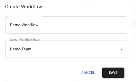
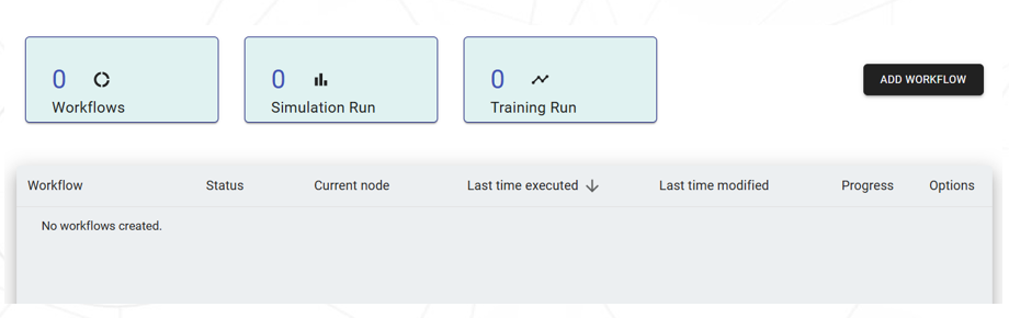
From the Dashboard, click Add Workflow.
Enter a name and pick the team that will own it.
Click Save. The workflow appears in the list.
Click its name to enter the canvas.

CREATE

EMPTY

SAVED

Adding nodes

Click the vertical AILog tab on the right edge of the canvas - it opens the AILog Nodes drawer.
You'll see two collapsible categories: Data Processing and AILog (the ML nodes).
Drag a node onto the canvas. Give it a name, click Save.
Double-click the node to open its Settings tab.

Connecting nodes

Hover over a node - a small connection handle appears at its top (target / input) and bottom (source / output).
Drag from the bottom handle of one node to the top handle of another to create a connection.
The canvas only permits valid connections - incompatible target nodes are grayed out while dragging.
Delete a connection by clicking it and pressing Delete.

CONNECT

Canvas controls

Action	How
Pan	Click and drag empty canvas
Zoom	Scroll wheel (0.2× – 10×)
Select	Click a node or edge
Multi-select	Hold `Shift` and click nodes
Copy / paste	Select items, then click the Copy and Paste buttons in the bottom-left toolbar (they appear only when something is selected)
Delete	Select + `Delete` key (confirmation dialog)
Run / Stop / Restart	Bottom-left toolbar - Start (▶), Stop (■, while running), Restart Workflow (↻)

Running & Monitoring

When every required node is fully configured, the Start button lights up. Execution is asynchronous - you can leave the page and come back.

Starting a run

Click the Start button (▶) in the bottom-left workflow toolbar.
Nodes without dependencies start first (level 0); everything downstream queues behind them.
Node colors change as they progress. Toasts pop up for each completion.
Click any finished (green) node to open its Results tab - plots, tables, and downloads.

Node status colors

Design

Being configured

Ready

Config complete

Waiting

In queue

Running

Processing now

Success

Completed · open results

Failure

Check error log

Stopped

Manually aborted

Stopping & re-running

Stop - click the Stop button (■) in the bottom-left toolbar while the workflow is running. Currently-executing nodes finish their step and halt.
Re-run - click Start again. Unchanged nodes skip to Success instantly (output is reused). Only nodes whose config changed re-execute.
Restart Workflow (↻) - wipes results from all succeeded nodes and re-runs from scratch. Useful when you want a clean re-execution; opens a confirmation dialog because it discards cached results.
Failed nodes - open the node, check the error panel, fix config, then click Start again. Successful ancestors stay cached.

★

Execution reuse saves hours on iterative ML work. Tweak Model Training parameters and re-run - Data Consolidation won't rebuild.

Node Reference

Click any card for full settings, results, and connection rules.

ALL NODES

DATA PROCESSING

AILog · ML

Workflow Patterns

Tested workflow design patterns you can copy. Drag these nodes, connect in order, configure, run.

★ Predict sonic logs on a blind well

The canonical synthetic-log workflow. Train on wells with DTC/DTS, predict where they're missing.

Data Consolidation → Log 10 Conversion → Model Training → Property Prediction

Time-indexed drilling data → depth-indexed training set

Convert EDR/MWD data from time to depth, then consolidate with existing logs for training.

Time to Depth → Data Consolidation → Model Training → Property Prediction

Full QC pipeline before training

Clean density, Vp/Vs, and slide artifacts before they poison your model.

Data Consolidation → Density Data QC → Vp/Vs Data QC → Slide Analysis → Model Training

★ Ahead-of-bit forecasting (LSTM-Convolution)

Drilling parameters drive a forward-looking log prediction. Lagged window pushes the prediction past the current bit depth. See the dedicated tutorial.

Time to Depth → Data Consolidation → Density / Vp-Vs QC → Model Training recurrent → Property Prediction

Unsupervised cluster model

Train a k-means cluster model on your log suite for facies / electrofacies discovery. Currently a terminal node - no downstream node on the AILog canvas consumes its output; the trained model is exported as a zip for use in other workflows.

Data Consolidation → Density / Vp-Vs QC → Model Training (Unsupervised) terminal

Iterative retraining

Tune model hyperparameters without re-processing data. Only Model Training and Property Prediction re-execute.

Data Consolidation cached → Model Training re-runs → Property Prediction re-runs

Tutorial · Your First Workflow

Consolidate two wells and plot the combined data. About 10 minutes.

1. Setup

2. Build

3. Configure

4. Run & Review

Prepare your data

Go to Data Management.
Create a folder named my-first-project.
Inside, upload two well CSV files. Each must have a depth column and at least a few log curves (e.g. GR, RHOB, DTC).
Confirm both files show up in the folder.

Build the canvas

Go to Dashboard → Add Workflow. Name it first-consolidation. Save.
Click the workflow name to enter the canvas.
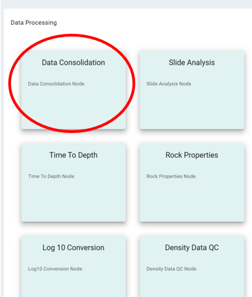
Click the AILog tab on the right edge of the canvas. In the drawer that opens, expand Data Processing.
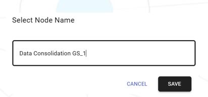
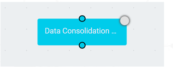
Drag a Data Consolidation node onto the canvas. Name it consolidate. Save.

NODES DRAWER

NAME NODE

ON CANVAS

Configure the node

Double-click the consolidate node to open its Settings tab.
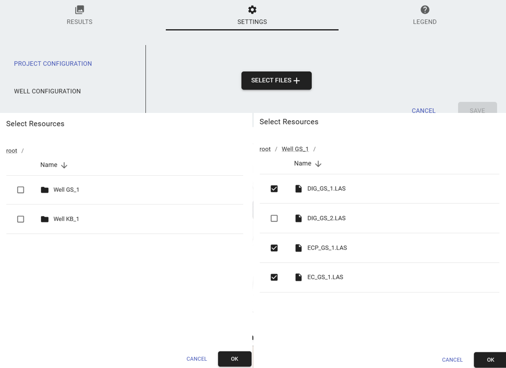
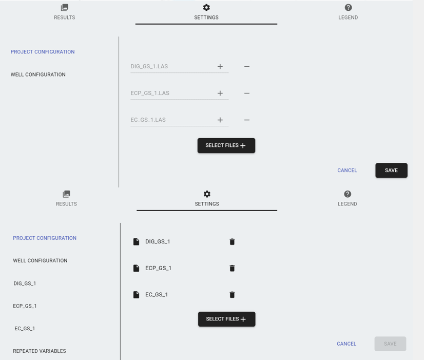
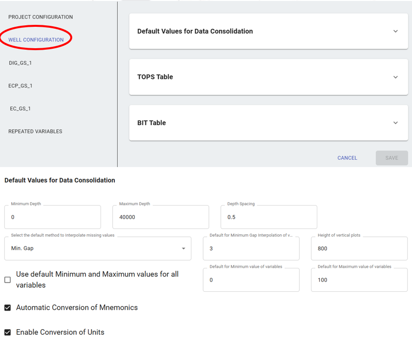
In the Project Configuration topic (left sidebar), click Select Files, navigate into my-first-project, and pick both CSVs.
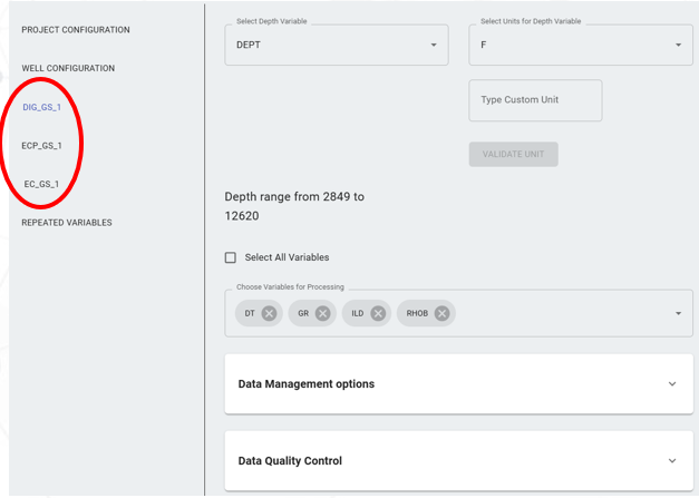
Open the Well Configuration topic and expand Default Values for Data Consolidation. Set Minimum Depth and Maximum Depth that cover both wells; leave Depth Spacing at 0.5.
Each loaded file gets its own topic (named after the filename). For each one, pick Select Depth Variable and use Choose Variables for Processing to keep the curves you want.
Close the panel. The node is now Ready - its status indicator (small dot in the top-right of the node) updates accordingly.

SELECT FILES

WELL CONFIG

VARIABLES

FILE SETTINGS

★

Leaving Auto Mnemonic Conversion on makes life easier when wells use different naming conventions (RHOZ vs RHOB, etc).

Run & review

Click Start (▶) in the bottom-left toolbar. The node's status indicator cycles grey (Waiting) → orange (Running) → green (Success).
When the indicator turns green, click the node to open the Results tab.
Download the consolidated CSV, or inspect the QC plots for each variable.

RUNNING

RESULTS

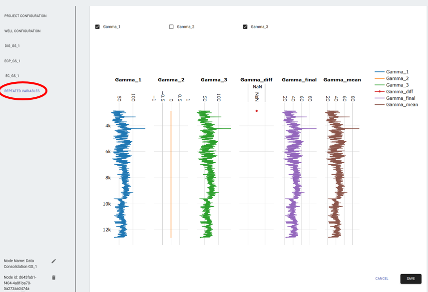
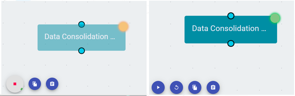
You now have a clean, combined dataset ready to feed into training, QC, or rock property nodes.

Tutorial · Train a Model & Predict

Extend your first workflow to produce a synthetic DTC log on a blind well. About 30 minutes depending on epochs.

1. Extend Canvas

2. Configure Training

3. Configure Prediction

4. Run & Compare

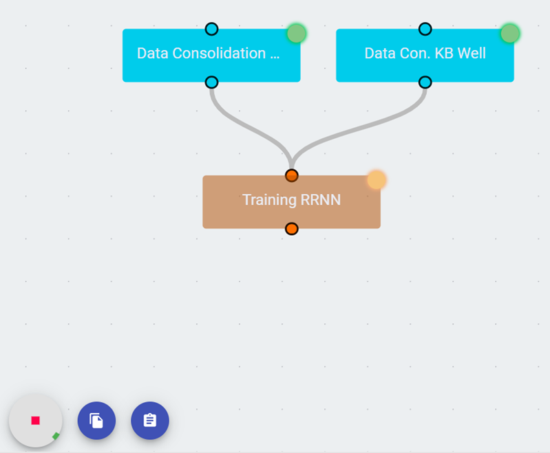
Add training and prediction nodes

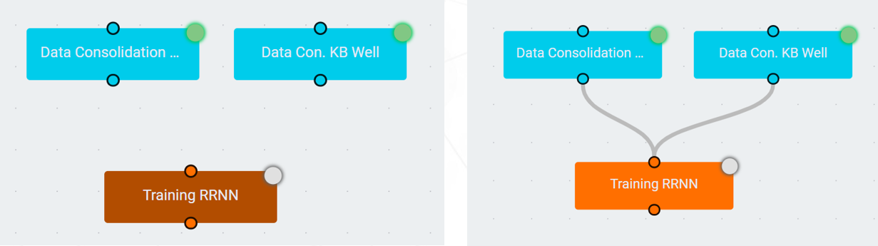
In your first workflow (or a copy), drag in a Model Training node from the AILog category.
Drag an edge from Data Consolidation into Model Training.
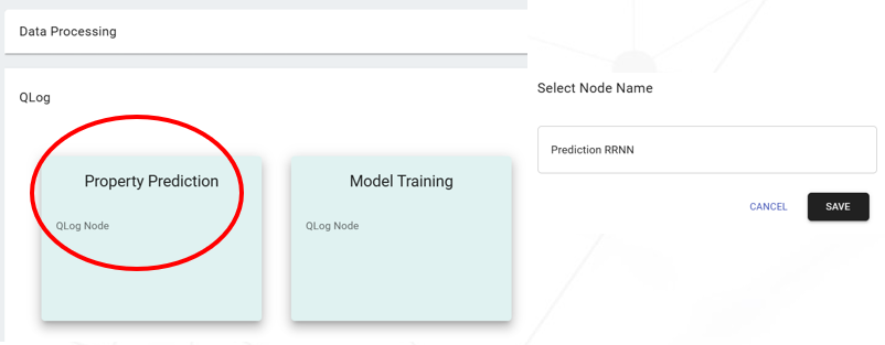
Drag in a Property Prediction node.
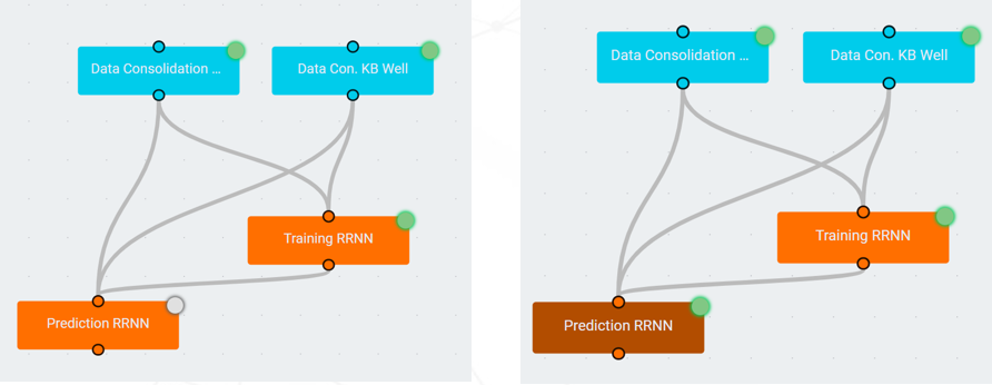
Connect Model Training → Property Prediction.
Optionally, drag a second edge from Data Consolidation → Property Prediction (so prediction knows which wells to score).

ADD NODE

CONNECT

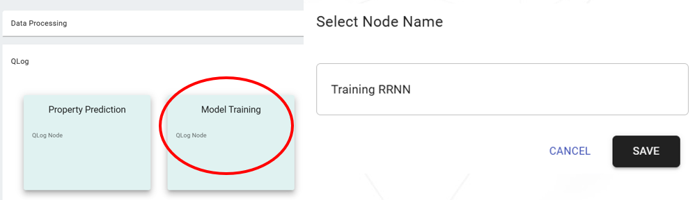
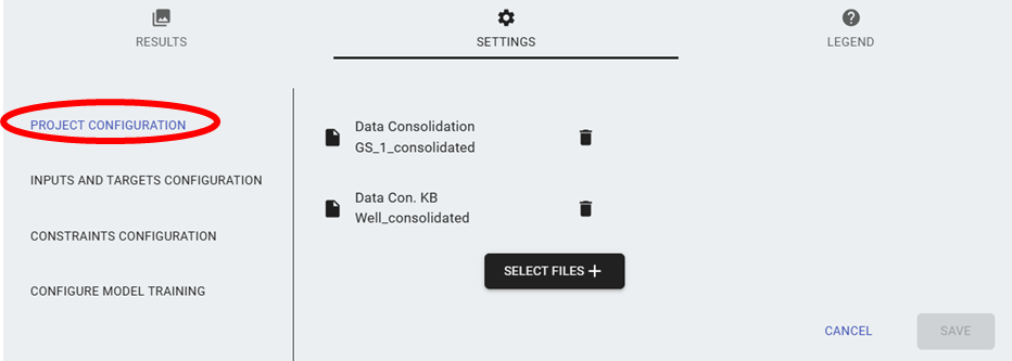
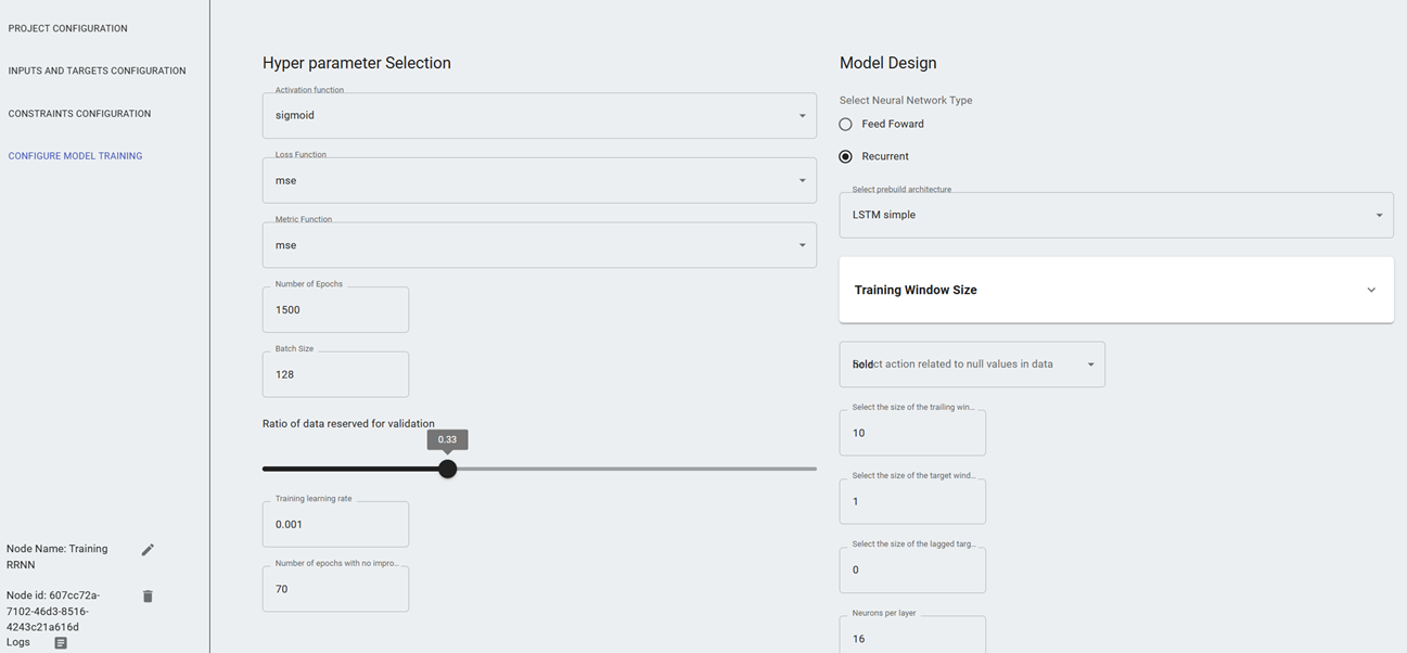
Model training settings

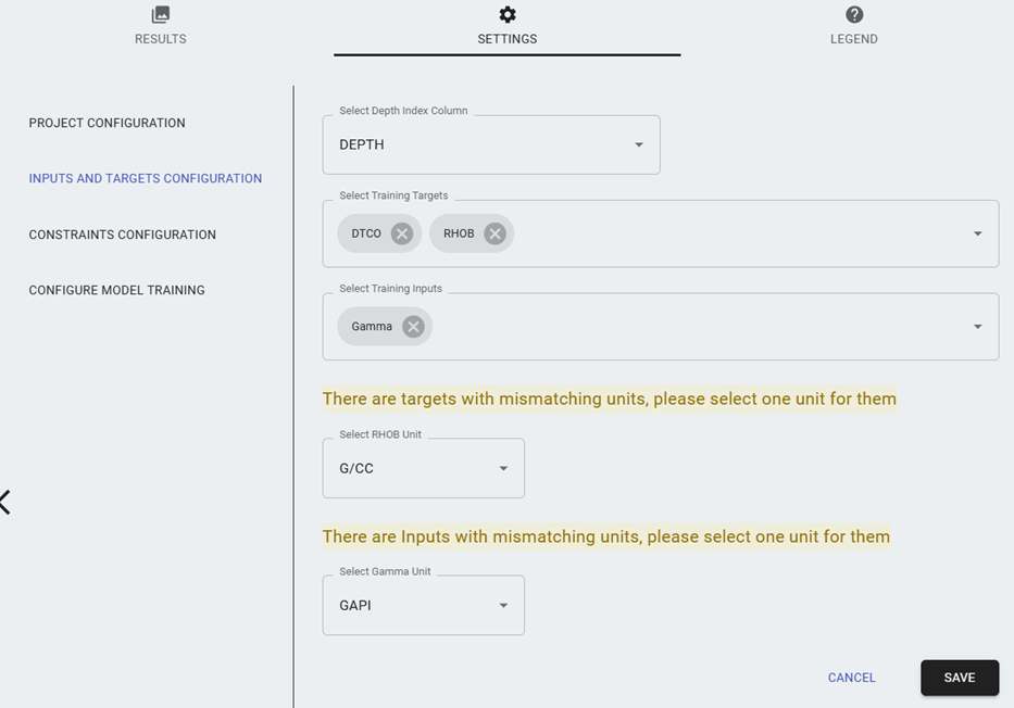
Double-click Model Training.
Training targets: pick DTC (or whichever curve you want to predict).
Training inputs: pick features you expect to correlate - GR, RHOB, WOB, SPP, etc.
Neural network type: start with Feed Forward; Architecture: Two Layer FFNN - fast, good baseline.
Epochs: 200 is a reasonable start. Batch size: 256.
Ensemble members: 5 - gives you an uncertainty band at predict time.
Leave loss, metric, and activation at defaults unless you know what you're doing.

★

Switching Neural network type to Recurrent exposes three extra knobs -trailing, target, and lagged windows. They're what make recurrent models powerful for depth-wise structure and ahead-of-bit forecasting. Read Recurrent Windowing before switching, and the ahead-of-bit tutorial for an end-to-end example.

INPUTS / TARGETS

MODEL CONFIG

ARCHITECTURE

TRAINING

RESULTS

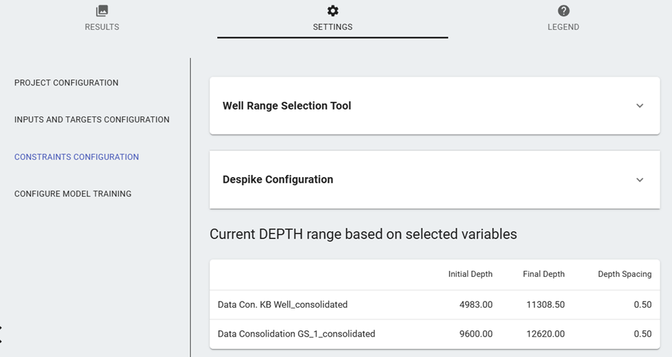
Property prediction settings

Double-click Property Prediction.
In Model Evaluation, inspect which wells were used for training - any not used is a candidate blind well.
Under Ensemble solution configuration, pick Use all ensemble for your first run (simplest).
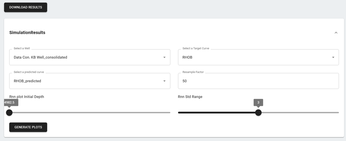
Under Simulation configuration → Simulation batch size, pick Data set length for FFNN models.

SETUP

EVALUATION

ENSEMBLE

SIM CONFIG

RESULTS

Ensembles give you an uncertainty band. If you trained N members, prediction is the mean across them and spread tells you where the model is uncertain.

Run and compare

Click Start (▶). Data Consolidation reuses its cached output (status indicator green immediately).
Model Training churns - its status indicator stays orange (Running) for minutes (depends on epochs and data size).
Property Prediction runs after training finishes.
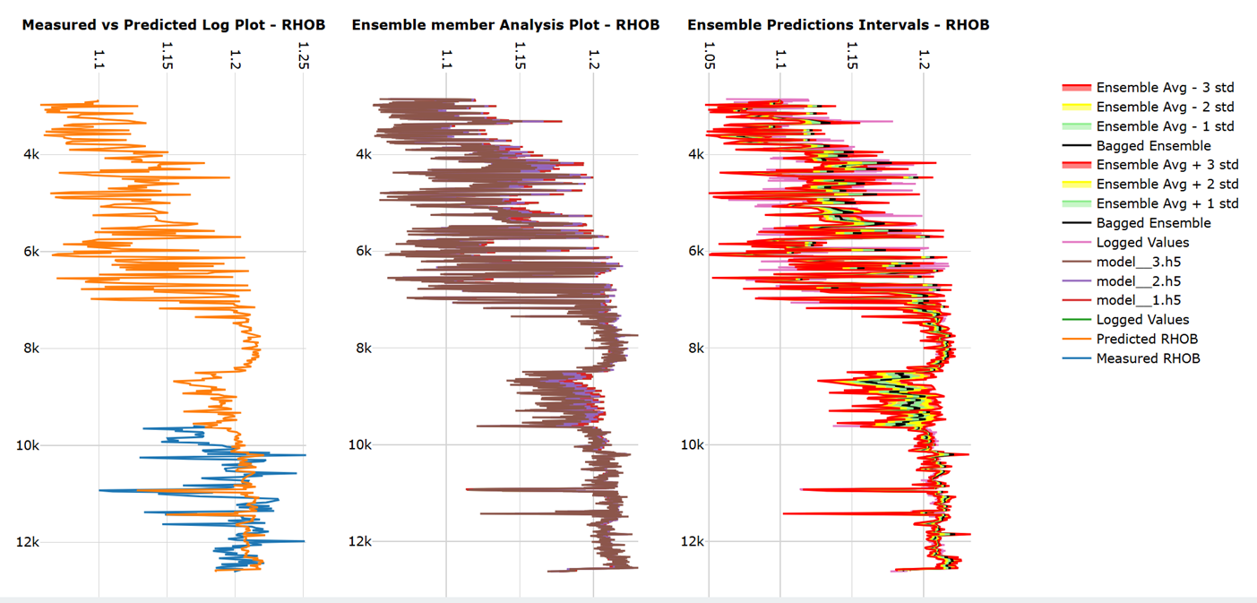
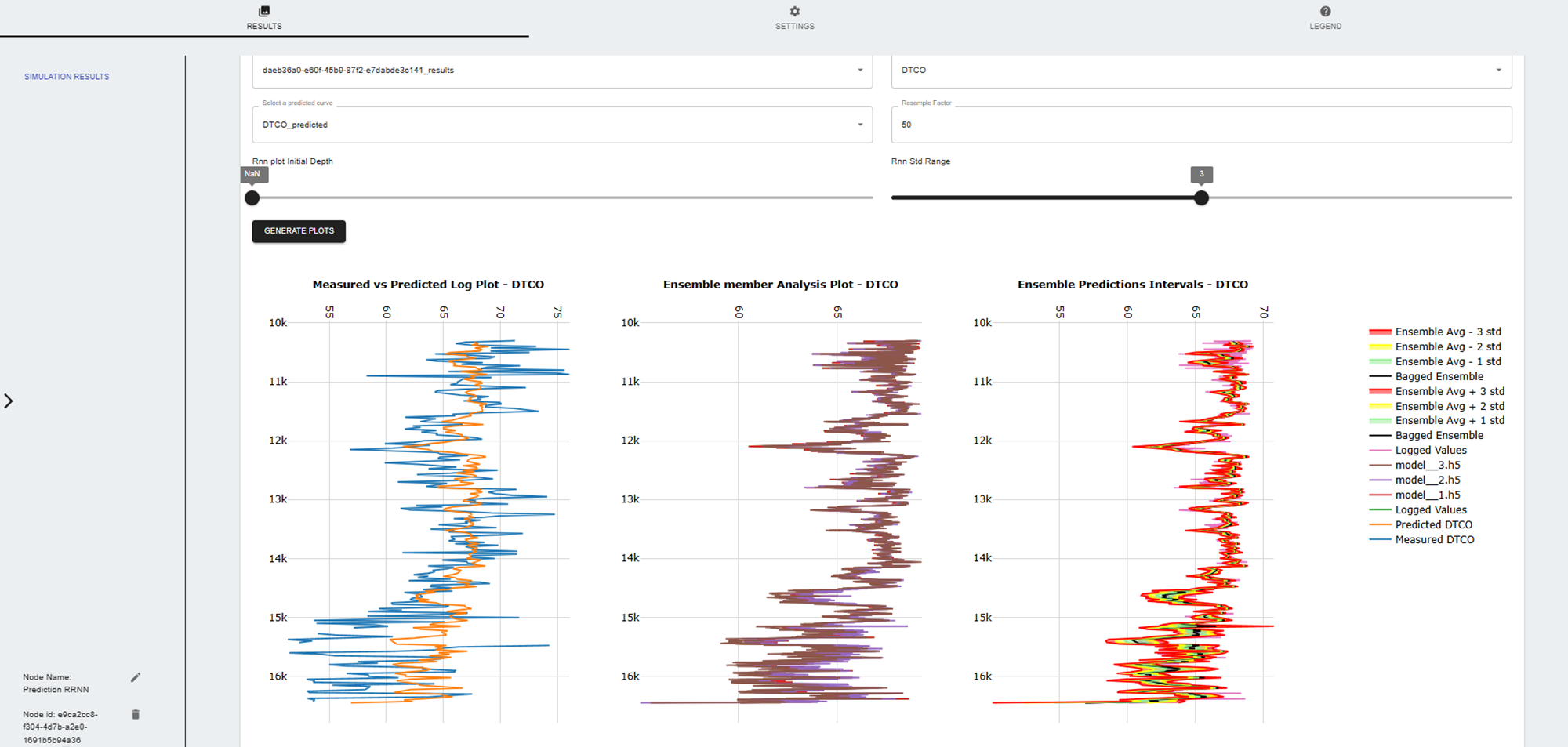
Open Property Prediction → Results. You get:
- Predicted log overlaid against ground truth (where available)
- Scatter plots of predicted vs actual
- Downloadable CSV with DTC_pred and DTC_std columns

★

If results look bad, tune training without touching upstream nodes. Re-runs reuse the consolidated data instantly.

Recurrent Windowing - Trailing, Target & Lagged Windows

Recurrent architectures (LSTM, LSTM-Convolution, TCN v2.0) read a window of samples at every step. For ahead-of-bit forecasting you tell the model three things: where each input sensor lives relative to the bit (the per-input window), how much drilling history to read (trailing window), how far ahead of the bit to predict (target window), and how to align behind-the-bit sensors with that ahead-of-bit target (lagged window).

Why this matters: drilling sensors don't all live at the bit

Drilling parameters - WOB, RPM, SPP, TOR, ROP - are measured at the bit itself.
Behind-the-bit sensors - MWD gamma, resistivity, MWD telemetry curves - sit on the BHA a known number of depth samples behind the bit. Gamma is commonly ~30–40 samples behind, depending on tool placement.

The recurrent windowing controls let you tell the model exactly where each input was sampled, and where you want the prediction to land - typically several samples ahead of the bit.

★

Worked example we'll use throughout this section: gamma sensor sits 40 samples behind the bit; we want to forecast gamma 30 samples (~15 ft at 0.5 ft spacing) ahead of the bit using 80 samples of drilling history.

The four knobs

Per-input window (set in "Training Window Size", per input variable)

The position of each input sensor relative to the bit, in samples.

Drilling variables (WOB, RPM, SPP, ROP, TOR): set to 0 - they are recorded at the bit.
Gamma (40 samples behind the bit): set to -40. The negative sign means "behind the bit".
Any other behind-the-bit sensor: set to -N, where N is the physical sample offset.

For recurrent models the slider stores a single offset value that applies to that input across the whole window. Uncheck Use same fixed window so each input can have its own offset.

Trailing window (min 4, max 128)

Number of previous drilling-data samples fed to the input layer at each step. Trailing = 80 with a 0.5 ft depth spacing means the model reads 40 ft of drilling history every time it makes a prediction.

Target window (min 1; max = trailing for TCN v2, max 128 otherwise)

Ahead-of-bit horizon - number of samples past the bit that the model predicts in one shot. Target = 30 with 0.5 ft spacing means each prediction step emits 15 ft of forecast curve. Target = 1 collapses to single-sample regression.

Lagged target window (min 0)

Aligns behind-the-bit inputs with the ahead-of-bit target. Set this to the absolute value of the most-negative per-input window. In the gamma example, gamma's per-input window is -40, so lagged = 40. If the only inputs you use are at the bit (window = 0 everywhere), lagged = 0 is correct.

The gamma example - full configuration

Field	Value	Meaning
Per-input window: `WOB`	`0`	WOB is recorded at the bit.
Per-input window: `RPM`	`0`	RPM is recorded at the bit.
Per-input window: `SPP`	`0`	SPP is recorded at the bit.
Per-input window: `ROP`	`0`	ROP is recorded at the bit.
Per-input window: `GR`	`-40`	Gamma sensor sits 40 samples behind the bit.
Trailing window	`80`	Use 80 past drilling samples as input context.
Target window	`30`	Predict 30 samples (~15 ft at 0.5 ft spacing) ahead of the bit.
Lagged target window	`40`	Matches \|gamma offset\| so the prediction aligns ahead of the bit.

The rules the UI enforces

If you set values that violate these rules, the lagged-window field shows the maximum allowed value and a message explaining which rule kicked in.

All recurrent models: lagged ≤ max(|per-input window|). You can't align the prediction further ahead than the deepest input offset you defined. In the gamma example, max |window| = 40, so lagged ≤ 40.
TCN v2.0 only - additional rule: lagged ≤ trailing − target. The TCN's internal Cropping1D layer needs the input segment to be at least as long as the output segment plus the lag. With trailing = 80 and target = 30, this allows lagged up to 50. Combined with the input-window rule, the effective cap in the gamma example is min(40, 50) = 40.
TCN v2.0 only: target ≤ trailing. The cropping layer cannot produce more output samples than were fed in.
All recurrent models: trailing ≥ 4. Shorter is too little context for the recurrent layers to be useful.

The lagged-window error message in the UI tells you which input set the cap. If it says "max input window size = 40 (from GR)", that's gamma. To predict further ahead than 40, you need a sensor with a larger offset - there's no magic fix in the lagged field alone.

Quick recipes

Goal	Per-input windows	Trailing	Target	Lagged
Per-sample synthetic log (DTC from wireline)	All inputs at `0`	16–32	1	0
Coherent short-segment synthetic log	All inputs at `0`	32	4–8	0
Ahead-of-bit gamma (40-sample sensor offset, 15 ft horizon)	Drilling = `0`, GR = `-40`	80	30	40
Ahead-of-bit gamma, longer horizon (~30 ft)	Drilling = `0`, GR = `-40`	128	60	40

Feed-Forward vs Recurrent - what the slider means

Feed Forward: the per-input window is a range of integer offsets. Negative reaches into the past, positive reaches forward. The model sees a flattened feature vector - no temporal recurrence - so trailing/target/lagged don't apply.
Recurrent: the per-input slider is a single offset (stored internally as [n, n]). Inputs are stacked into a 3-D tensor (batch, time, features), and trailing / target / lagged appear below the architecture box.

Tutorial · Ahead-of-Bit Prediction with LSTM-Convolution

Build a model that, while drilling, predicts the next several feet of log curve before the bit gets there. Drilling parameters (WOB, RPM, SPP, ROP) drive the prediction; the model produces a forward-looking gamma / sonic / density curve.

The trained model can later be reused for streaming forecasts at the rig. Same training math - the difference at runtime is that the inputs are streamed in sample by sample instead of read from a CSV.

1. Data Setup

2. Model Choice

3. Windowing

4. Train

5. Predict & Evaluate

Build the data

Start from a Time to Depth node - drilling data is recorded in time, but training is depth-indexed.
Feed the depth-indexed file into Data Consolidation together with any wireline / LWD logs you want as targets.
Run Density Data QC and Vp/Vs Data QC if your target is a sonic or density curve - bad logs are the #1 reason ahead-of-bit models fail.
The output of QC feeds a Model Training node.

Recommended chain

Time to Depth → Data Consolidation → Density / Vp-Vs QC → Model Training → Property Prediction

Pick the architecture

For ahead-of-bit prediction you want a model that can (a) read a window of drilling parameters, (b) extract local patterns at multiple resolutions, and (c) emit a coherent short curve segment ahead of the bit. The LSTM-Convolution v1.0 architecture is purpose-built for this - Conv1D layers extract local drilling-pattern features, max pooling compresses them, and a stacked BiLSTM models long-range structure before a dense output.

Open Model Training.
Under Model Design → Neural Network Type, pick Recurrent.
Under Architecture, pick LSTM-Convolution v1.0.
Set Filters = 32, Kernel size = 10, Pool size = 3 for a sensible starting point.

★

TCN v2.0 is a faster alternative - pure dilated causal convolutions. Use it if training time matters more than the last 5% of accuracy.

Configure the windows - gamma example

We'll build the canonical ahead-of-bit configuration: gamma sensor 40 samples behind the bit, drilling parameters at the bit, predict 30 samples (15 ft) ahead. Once you understand this layout you can adjust offsets and horizons for your own BHA.

Training inputs - drilling parameters at the bit: WOB, RPM, SPP, TOR, ROP; plus the behind-the-bit sensor we'll forecast: GR (or whichever MWD curve you have).
Training targets - pick the curve we want to forecast ahead of the bit: GR.
Open Training Window Size and uncheck "Use same fixed window". Each input now gets its own slider - its physical position relative to the bit, in samples.
Set the per-input windows:
- WOB: 0 (at the bit)
- RPM: 0 (at the bit)
- SPP: 0 (at the bit)
- TOR: 0 (at the bit)
- ROP: 0 (at the bit)
- GR: -40 (gamma sensor sits 40 samples behind the bit - adjust to your BHA's actual offset)
(Set Max window size to 40 or higher so the GR slider can reach - 40.)
Below the architecture box, set the recurrent windowing:
- Trailing window = 80 - read 80 past samples (40 ft at 0.5 ft spacing) of drilling data as input context.
- Target window = 30 - predict 30 samples (15 ft at 0.5 ft spacing) ahead of the bit per step.
- Lagged target window = 40 - matches |gamma offset| so the predicted segment lands ahead of the bit instead of at the gamma sensor depth.
Scaling I/O: (0, 1) usually works best for drilling parameters since most are non-negative.
Null action: interpolate or hold - drilling streams have brief gaps; don't let nulls poison the recurrent layers.

The simple rule for lagged is: lagged = |most-negative per-input window|. If your only behind-the-bit sensor is gamma at -40, lagged = 40. If you also have a resistivity tool 60 samples behind the bit (window -60), lagged becomes 60 and every behind-the-bit input contributes to the same alignment.

If you switch to TCN v2.0 the rules tighten. The lagged field will cap itself at min(|max input window|, trailing − target) and the target field caps at trailing. With trailing = 80 and target = 30 those second rules don't bite (50 ≥ 40), but if you ever raise target or shrink trailing the UI will stop you with an explicit message naming the rule.

Train

Epochs: 300 is a reasonable starting point for a single-well training set; 1000+ for multi-well datasets.
Batch size: 64–128. Recurrent models are memory-hungry per sample.
Validation split: 0.2.
Early stopping patience: 30 epochs.
Ensemble members: 5–10. Each member is trained independently; the spread is your uncertainty band at runtime.
Dropout: yes, rate 0.05–0.10. Helps avoid memorizing the few wells you have.
Click Start (▶). Expect 10× the training time of a comparable FFNN - recurrent models are slower.

Predict and check

Drag a Property Prediction node from the trained Model Training.
Pick a hold-out well - one the model never saw. Connect it from Data Consolidation.
Set Ensemble solution → Use all ensemble.
Set Simulation batch size → Fixed size. For seq2seq models this controls how many windows are evaluated per chunk; Data set length doesn't fit in memory.
Click Start. Inspect:
- Predicted curve on the test well, overlaid with ground truth.
- Per-depth uncertainty (ensemble standard deviation). Wide bands = the model is guessing.
- Scatter plot of predicted vs actual. The closer the diagonal, the better.

★

The trained model can be exported and reused at the rig for streaming forecasts. Drilling parameters arrive sample by sample, the model re-runs every step and slides the prediction window forward. The lagged window you trained with is exactly the look-ahead distance the rig sees in real time.

FAQ & Tips

Common questions, answered.

Why is my node still in Waiting / not running?

The node is in Waiting - it's been queued and is waiting for a free CPU slot on the server. Large workflows queue nodes level-by-level; the status indicator turns orange (Running) as soon as a worker is available.

The Start button is grayed out. Why?

At least one node in the workflow is not fully configured - it's still in Design. Open any gray node, complete its required fields, close it, and Start will light up.

My edge won't connect between two nodes.

The canvas enforces connection rules per node type. Rock Properties, for example, only accepts one upstream edge and only feeds into Log Data QC. Check the Node Reference for each node's valid inputs and outputs.

I changed the training config, but the workflow finished instantly.

Cache hit. AILog fingerprints each node's config; if the fingerprint hasn't changed, the prior output is reused. Scroll to the node's config - something you thought you changed may have snapped back to a default. Toggle a value and click Start again.

Can I share a workflow with another team?

Not directly - workflows are team-scoped. But an admin can copy a workflow's configuration into another team, or add a user to both teams so they can see and copy it manually.

What happens if a node fails mid-workflow?

The failed node's status indicator turns red; downstream nodes stay in Ready. Fix the config or data, then click Start again. Upstream successes remain cached, so you only pay for the failed node and its descendants.

How do I pick the right neural network architecture?

Start with Two Layer FFNN - it's fast and often good enough. If log predictions are "jittery" and you suspect depth-wise dependencies matter, try LSTM v1.0 or TCN v2.0. Recurrent models take longer to train but capture long-range structure. For ahead-of-bit forecasting, use LSTM-Convolution v1.0 with a non-zero lagged window - see the ahead-of-bit tutorial.

What's the difference between trailing, target, and lagged windows?

Trailing = how many past drilling-data samples the model reads as input. Target = the ahead-of-bit horizon, i.e. how many samples past the bit the model predicts in one shot. Lagged target window = the absolute value of the most-negative per-input window, used to align behind-the-bit sensors (gamma at -40 ⇒ lagged = 40) with the ahead-of-bit prediction. If every input is at the bit (window 0), lagged = 0 is correct. Full walkthrough with the gamma example: Recurrent Windowing.

Why does the lagged target window field show "Maximum value is N"?

For all recurrent models: lagged ≤ max(|per-input window|) - you can't align further ahead than the deepest sensor offset you defined. For TCN v2.0 only, two extra rules: lagged ≤ trailing − target (Cropping1D needs input ≥ output + lag) and target ≤ trailing. The error message names the input or rule that capped you, so you know which number to bump.

When should I use Model Training (Unsupervised) instead of Model Training?

Use the unsupervised node when you don't have target curves to predict - for facies / electrofacies discovery, reservoir characterization, or anomaly flagging. It's k-means at heart: pick a feature set (GR, RHOB, NPHI, RT, …), let it cluster the depth samples, and use the elbow plot to validate your k. The node is terminal on the AILog canvas - no other node consumes its output. The trained cluster model is exported as a zip for downstream use outside AILog.

Where do my downloaded results come from?

Every node keeps an output folder per execution. When you download from a node's Results tab, it zips that folder and streams it to your browser.

Glossary

Quick definitions of terms you'll encounter.

Workflow

A saved chain of connected nodes that together accomplish a task (consolidate → train → predict, etc.).

Node

A single processing step on the canvas - has a config, produces an output, passes data downstream.

Edge

A connection between two nodes. Edges carry data from an upstream node's output into a downstream node's input.

Mnemonic

A short name for a log curve - GR, RHOB, DTC, DTS, NPHI, etc.

Blind well

A well held out from training so you can compare predicted logs to actual ground truth.

Ensemble

A group of N trained models whose predictions are averaged. Spread across members = uncertainty.

DTC / DTS

Compressional / shear sonic slowness - core velocity curves.

RHOB

Bulk density log (g/cm³).

Gamma ray - proxy for shale content and lithology.

Vp/Vs

Ratio of compressional to shear velocity. Indicator of rock type and fluid.

WOB / SPP / TOR / RPM

Drilling parameters: weight on bit, stand pipe pressure, torque, rotations per minute.

Tops

Stratigraphic formation tops - depths where geologic units begin.

Checkshot

Time-depth calibration used for the Time to Depth conversion.

DCAL

Differential caliper - borehole size used in density QC.

Epoch

One full pass through the training dataset. More epochs = more learning (until overfitting).

Early stopping

Halt training when the validation metric stops improving for a set number of epochs (patience).

FFNN / LSTM / TCN

Feed-Forward Neural Net · Long Short-Term Memory · Temporal Convolutional Network. The three model families AILog supports.

Trailing window

Number of past drilling-data samples fed to the recurrent input layer at each step (4–128). Larger = more context, more compute.

Target window

Ahead-of-bit horizon - number of samples past the bit the model predicts in one shot. Target = 1 collapses to single-sample regression; target > 1 emits a coherent short forecast segment.

Lagged target window

Alignment offset for behind-the-bit sensor inputs. Set to the absolute value of the most-negative per-input window (e.g. gamma at - 40 ⇒ lagged = 40), so the predicted segment lands ahead of the bit.

Per-input window

Position of an input sensor relative to the bit, in samples. Drilling parameters at the bit = 0; behind-the-bit sensors get a negative offset matching their physical placement on the BHA.

Conv1D

1-dimensional convolution. In LSTM-Convolution, used to extract local depth-wise patterns before feeding the BiLSTM stack.

Dilation (TCN)

Spacing between samples a convolution kernel reads. Stacked dilations let TCNs see far back without exploding parameter count.

k-means

Algorithm behind Model Training (Unsupervised). Partitions data into k clusters by minimizing within-cluster variance.

Elbow method

Plot of within-cluster variance vs k. The "elbow" - the point where adding more clusters gives diminishing returns - is a sensible choice for k.

Electrofacies

Cluster of depth samples whose log signature is similar enough to act as a proxy for a lithofacies. Output of Model Training (Unsupervised) is a per-depth electrofacies label.

Despike

Remove spurious spikes from a log curve using a statistical window.

Slide zone

A section drilled by sliding (no rotation) - logs often show characteristic artifacts here.

Scaler

Function that normalizes values into a standard range (MinMax: 0–1, Standard: mean 0 std 1).